What is a neural network? It is a term that gets thrown around a lot. What is it really? How does it work? Here, I am going to implement a simple neural network from scratch in Python with thoughts along the way.

---

I want to hop in to implementation details directly. But to do that I want to cover some background. Many of us have thought about intelligence and drawn connections to human brain. As the terms intelligence and human brain go hand in hand. We tried to mimic the human brain and understand the brain. The perceptron model, introduced by Frank Rosenblatt in the 1950s, was one of the prevalent models inspired by the brain. Later work was based on this model.

What we initially called perceptron is now called more generally as Neuron. Which, if we're talking about human biology, would mean the nerve cell in the brain. But in computer science we mean a function where it takes an input and generates a number as output.

The input is a combination of what we call weights and biases (weights are multiplied by input from previous layer). They are parameters so to speak. The weights are multiplied by the inputs and then added to the bias. Then this sum is passed through an activation function to produce the output of the neuron.

$$output = activation\_function(\sum{(weights * inputs)} + bias)$$

A Neural Network is a collection of these neurons that are connected together. Each neuron branches out to multiple neurons in the next layer. So there are a lot of connections. A layer is a collection of neurons that are at the same depth.

Training a neural network

When we initialize a neural network, the weights and biases are set at random. So the output of the network is random. To make the network useful, we need to adjust the weights and biases based on the input data and the expected output. This is where training comes in.

The process of finding the right weights and biases is called training. Now there are techniques for training a neural network. I won't go into the details of these techniques. But the most common technique is called backpropagation, which is what I will implement here.

Basic implementation

With that said, here is the implementation of a neural network in Python and then I will show how to train it to infer the curve of a sine wave

Neuron class

First we start with the implementation of the Neuron class. In my implementation the neuron takes a list of ancestors as input. The ancestors are the neurons in the previous layer that are connected to this neuron. The weights and biases are initialized at random.

The highlight of the neuron class is the activate method where it activates the neuron and the get_inputs method where it gets the inputs from the ancestors. It is sort of a recursive function that calls itself to get the inputs from the ancestors until it reaches the input layer.

The ABC thing is Python's way of doing abstract classes.

from abc import ABC, abstractmethod
import random
import math


class Neuron(ABC):
    def __init__(self, ancestors):
        self.ancestors = ancestors
        self.bias = random.uniform(-0.5, 0.5)
        self.weights = [random.uniform(-0.5, 0.5) for _ in ancestors]
        self.last_activation = None

    def activate(self):
        if self.last_activation is None:
            weights_sum = self.get_inputs()
            act = self.activate_function(weights_sum)
            self.last_activation = act
            return act

        return self.last_activation


    def get_inputs(self):
        weights_sum = self.bias
        for neuron in self.ancestors:
            weights_sum += (
                self.weights[self.ancestors.index(neuron)] * neuron.activate()
            )

        return weights_sum

    @abstractmethod
    def activate_function(self, x):
        pass

    @abstractmethod
    def activate_function_prime(self, x):
        pass

There are many types of activation functions, some of them are sigmoid, linear function, and Tanh. Linear is the simplest one but it is not suitable for our use case. Because it will make the output linear. Sigmoid is another function that is non linear but it is bounded between 0 and 1. Tanh is a non linear function that is bounded between -1 and 1. Because of the nature of the sine wave where it oscillates between -1 and 1. The tanh function is a good fit for our use case.

So here the implementation of the TanhNeuron where it implements the activate_function and activate_function_prime methods.

class TanhNeuron(Neuron):
    def activate_function(self, x):
        return math.tanh(x)

    def activate_function_prime(self, x):
        return 1 - math.tanh(x) ** 2

NeuralNetwork class

Then here comes the implementation of the NeuralNetwork. The neural network takes a list for the count of neurons in each layer. If we specify the shape of the network as [3, 4, 1] then it will create a network that takes 3 inputs and has 4 neurons in the middle (hidden layer), and 1 neuron in the output layer. Different applications of neural networks will have different shapes of networks.

infer method is the method that takes the inputs and returns the outputs.

class NeuralNetwork:
    def __init__(self, layer_sizes, neuron_type=TanhNeuron):
        self.layers = []
        prev_layer = []

        for layer_size in layer_sizes:
            current_layer = self.createLayer(layer_size, prev_layer, neuron_type)
            self.layers.append(current_layer)
            prev_layer = current_layer

    def createLayer(self, count, prev_layer, neuron_type):
        neurons = []
        for i in range(count):
            neurons.append(neuron_type(prev_layer))

        return neurons

    def set_inputs(self, inputs):

        for layer in self.layers:
            for index, neuron in enumerate(layer):
                neuron.last_activation = None

        for index, neuron in enumerate(self.layers[0]):
            neuron.last_activation = inputs[index]

    def infer(self, inputs):
        self.set_inputs(inputs)
        return [out.activate() for out in self.layers[-1]]

We set up everything for the network to be able to give us predictions. But if we run the network with the existing code, it will give us random predictions. This is because as said earlier the weights are set at random when we initialize the network.

Training the network

This is where the train method comes in. The method is quite involved and what I am doing here is implementing the backpropagation technique. The thing here is that this can be seen as "black box" or something can be replaced with a different algorithm. It is not crucial for the network to run, we could import the weights and biases in a different way to make predictions. But here is I will provide the implementation anyway for the competence.

def train(self, learning_rate, batch):
    for inputs, targets in batch:
        # Forward pass
        outputs = self.infer(inputs)

        # Calculate output layer errors
        output_errors = []
        for i, target in enumerate(targets):
            error = target - outputs[i]
            output_errors.append(error)

        # Backpropagation
        layer_errors = [output_errors]

        # Calculate errors for hidden layers (backward)
        for layer_idx in range(len(self.layers) - 2, 0, -1):
            current_layer = self.layers[layer_idx]
            next_layer = self.layers[layer_idx + 1]
            next_errors = layer_errors[0]

            current_errors = []
            for neuron_idx, neuron in enumerate(current_layer):
                error = 0.0
                for next_neuron_idx, next_neuron in enumerate(next_layer):
                    error += next_errors[next_neuron_idx] * next_neuron.weights[neuron_idx] * next_neuron.activate_function_prime(next_neuron.get_inputs())
                current_errors.append(error)

            layer_errors.insert(0, current_errors)

        # Update weights and biases
        for layer_idx in range(1, len(self.layers)):
            layer = self.layers[layer_idx]
            errors = layer_errors[layer_idx - 1]

            for neuron_idx, neuron in enumerate(layer):
                # Update weights
                for weight_idx, ancestor in enumerate(neuron.ancestors):
                    gradient = errors[neuron_idx] * ancestor.activate() * neuron.activate_function_prime(neuron.get_inputs())
                    neuron.weights[weight_idx] += learning_rate * gradient

                # Update bias
                bias_gradient = errors[neuron_idx] * neuron.activate_function_prime(neuron.get_inputs())
                neuron.bias += learning_rate * bias_gradient

Backpropagation calculates the difference between the network's output and the desired result, then works backward to tweak weights and biases to reduce this error. Think of an old radio, where each weight and bias is a dial. When you tune a dial, you hear more or less static. Backpropagation is similar, it measures the static and adjusts each dial based on how much it contributes to the noise. If the predicted output is too different than the actual value, it will add a value to make nearer to desired output. With each tweak, the static fades, and the network's predictions gets closer to the true output.

Putting it all together

Now let's see how to actually use our neural network classes to solve a real problem. We'll train it to learn the sine wave function, a classic example that shows how neural networks can approximate mathematical functions.

First, we create our neural network. We want it to take one input (the x value) and produce one output (the sine of x). We'll use a hidden layer with 4 neurons, this gives the network enough capacity to learn the sine wave without being too complex:

# 1 input -> 4 hidden neurons -> 1 output
network = NeuralNetwork([1, 4, 1])

Next, we need training data. We'll generate points along the sine wave from -π to π. For each x value, our target output will be sin(x). We create a list of tuples, where each tuple contains the input and the expected output:

import math

training_data = []
for i in range(100):
    x = -math.pi + (2 * math.pi * i / 99)
    y = math.sin(x)
    training_data.append(([x], [y]))

Now comes the training. We'll train for 1000 epochs (complete passes through our data) with a learning rate of 0.01. During each epoch, we show the network all our training examples and let it adjust its weights and biases:

print("Training neural network...")
for epoch in range(1000):
    network.train(0.01, training_data)

    if epoch % 100 == 0:
        test_points = [-math.pi, -math.pi/2, 0, math.pi/2, math.pi]
        total_error = 0
        for x in test_points:
            predicted = network.infer([x])[0]
            actual = math.sin(x)
            error = abs(predicted - actual)
            total_error += error
        avg_error = total_error / len(test_points)
        print(f"Epoch {epoch}: Average error = {avg_error:.6f}")

After training, let's see how well our network performs:

print("\nFinal predictions:")
test_points = [-math.pi, -math.pi/2, 0, math.pi/2, math.pi]
for x in test_points:
    predicted = network.infer([x])[0]
    actual = math.sin(x)
    print(f"sin({x:.2f}) = {actual:.4f}, predicted = {predicted:.4f}")

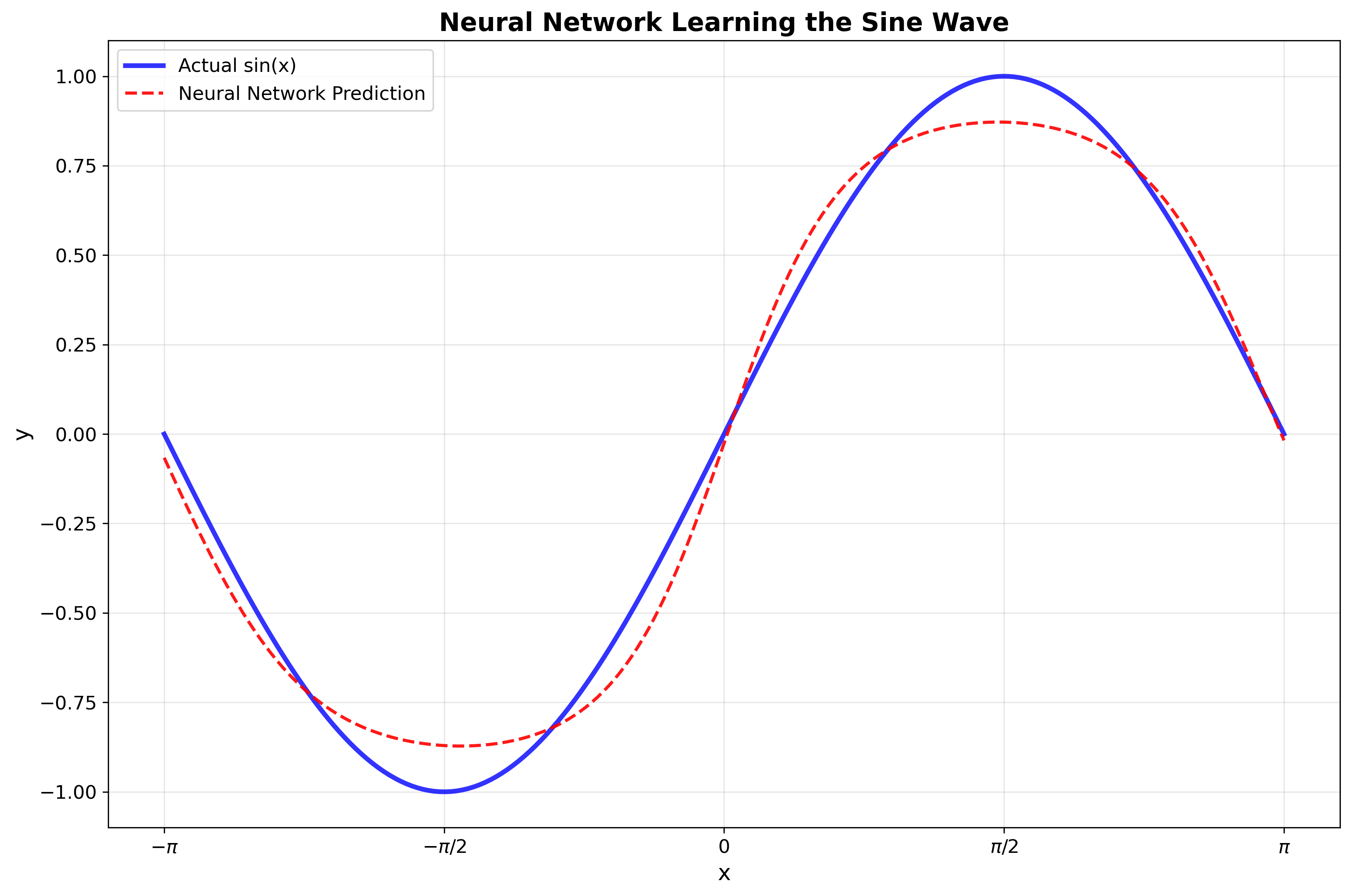
Running this code, you'll see the error decrease over time as the network learns. By the end, it should predict sine values quite accurately (maybe not perfectly), but close enough to show it understands the pattern of the sine wave.

Below is the graph of the predictions of the neural network against the actual sine wave, when I ran the code.

Discussion

Our neural network implementation is embarrassingly simple, yet it can theoretically approximate many functions given enough neurons. What's fascinating is how little we actually need to understand to build something that works. We don't need to deeply understand or know how all parameters interact, we just need to implement the network and a training algorithm. The network will figure out the rest through training.

This implementation here could be the foundation for something that recognizes images, translates languages, or plays games at superhuman levels. Not because it's particularly clever, but because it's a decent approximation of a very general computing pattern.